Discrete Fracture Network

DFN Block Analyser

Project Setup

In this window you define the geometry for the excavation surface that you will analyse, and the volume of the DFN.

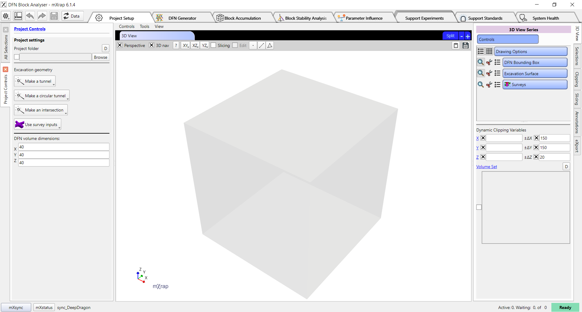
Project folder: specifies a folder to store the accumulated blocks for this project. You can open the project again at a later date to continue stability analysis using the accumulated blocks. Note that you can only accumulate new blocks if your excavation geometry matches the previous excavation geometry, we recommend saving a workspace of your project to save the excavation geometry settings, project folder, and selected DFN parameters file.

The excavation geometry can be based on survey files (e.g. your own designs or asbuilts), or it can be created according to preset shapes: tunnels, circular tunnels, or intersections. In the current version, only the non-circular tunnel option can be used with ground support standards.

If you click on the tunnel, circular tunnel, or intersection options then the control panel will update to show input parameters for the geometry.

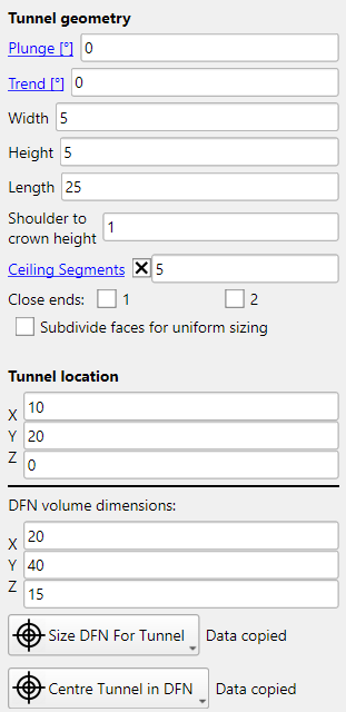
Plunge: defines the plunge of the tunnel (or one axis of the intersection). Plunge is always in the direction of trend.
Trend: defines the trend of the tunnel.
Width: defines the width of the tunnel.
Height: defines the height of the tunnel, from the floor to the crown.
Length: defines the length of the tunnel.
Shoulder to crown height: used for creating arched backs, specifies the height of the arch.
Ceiling segments: specifies the number of segments used when creating arched backs. More segments will create a smoother arch, but will increase the processing time of block accumulation.
Close ends: controls whether the end of the tunnel is closed or open. If a tunnel has a closed end that is within the DFN volume, then blocks may accumulate on the end. This may be useful if you wish to analyse block formation on the face, but there are limited tools for this analysis at this time.
Subdivide faces for uniform sizing: we recommend turning this option off for the block analyser. The subdivision of faces will increase the processing time of block accumulation, and provides no benefit for this application.
Tunnel location: specifies the coordinates of the centre of the floor of the tunnel.
DFN volume dimensions: specifies the volume that joints will be generated in.

The Size DFN For Tunnel button can be used to quickly resize DFN volume and place the tunnel in the middle of the volume. It usually provides a reasonable default, but you may wish to customise the location or volume according to your use case.

Joints are only generated within the DFN volume, so the DFN volume must extend far enough around your excavation surface to capture the largest blocks that you could anticipate. Note that the edge effect of joint generation is already mitigated by the DFN generator, so you do not need to oversize your DFN volume to account for edge effects. The larger the DFN volume is, the more time that DFN generation will take and the more time that block finding will take.

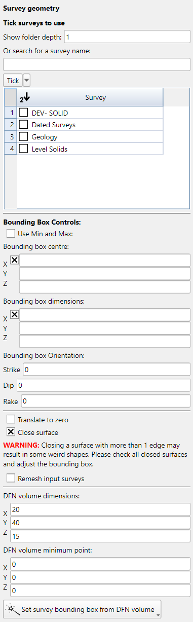
If you click on Use survey inputs then the control panel will update to show you settings for selecting a survey, clipping and optionally remeshing the survey, and positioning the DFN volume.

The following is a good process to follow for using survey inputs. First, in the 3D View Series controls, turn off the DFN Bounding Box and Excavation Surface, then turn on the Surveys series. In the Surveys series options, turn on the survey that you want to use. Then click on the 3D View and press the R button to reset the view.

You should now be able to see your surveys. You can zoom in to an area of interest by hovering the mouse over a point on the surveys and pressing the F key. Once you have found an area of interest, we want to position the DFN volume there. There are two convenient ways to find the coordinates:

Using the annotations tool, place a point on the survey and then read the coordinates of that point.
Turn off Perspective in the 3D view, then use the XY, XZ, YZ buttons to align the view so that you can read the coordinates from the grid.

Now, turn on the DFN Bounding Box series and then type your coordinate in the DFN volume minimum point input at the bottom of the panel. You should see the transparent grey box indicating the DFN volume. Adjust the minimum point and the volume dimensions to cover your area of interest.

When you have the position correct, turn off the Surveys series and turn on the Excavation Surface series. Now tick the survey in the table in the control panel on the left. To begin with you should see all of the survey, but we want to clip the survey to the area of interest so that the block finding process will be more efficient. At the bottom of the control panel click on the Set survey bounding box from DFN volume.

By default the surface is clipped exactly to the DFN volume, and also closed by attempting to automatically fill any holes in the survey. We will adjust our bounding box minimum and maximum so that the clipping area is slightly larger than the DFN volume, and we will untick the Close surface option.

If your surveys have quality issues such as internal surfaces, holes, self-intersections, or non-manifold topology then they will cause problems with the block-finding process. There is an integrated remeshing option which can fix some of these problems. To enable it, tick the Remesh input surveys option in the control panel. If the remesher fails or there are still quality issues then you will need to correct your input surveys in external software.

DFN Generator

This window is for configuring the DFN generation. You should already have calibrated DFN parameters from the DFN Generator app, so we will simply select the CSV containing those parameters for the DFN Input Parameters in the top of the left-hand control panel.

Block Accumulation

In this window we will create many different DFN realisations from our DFN input parameters. For each DFN realisation the app will search for tetrahedral blocks which form on the outside of the excavation surface, and then save those blocks into the project folder.

First we click the Initialise analysis button. Warning: this will clear any existing data in this project folder. This also saves the excavation shape into the project folder.

After the project folder has been initialised you should see additional controls with an input for the Number of DFNs to generate, and a button to Run analysis. If we set 10 DFNs to generate and click the button, then the block finding process will run for 10 DFN realisations.

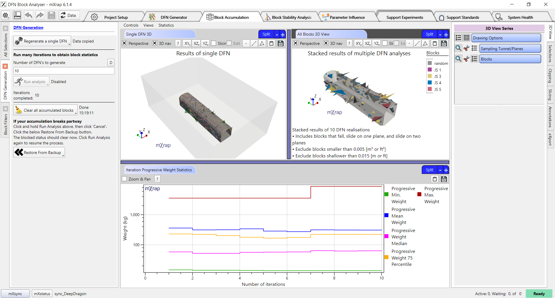
The Single DFN 3D view shows the blocks found for the current DFN realisation. The All Blocks 3D View shows all blocks that have been saved into the project folder. At the bottom of the screen the Iteration Progressive Weight Statistics chart shows statistics about the accumulated block weights, calculated progressively across all runs. For example, the mean weight line at X=5 will show the mean weight of all blocks from the first 5 DFN realisations. We want to run enough DFN realisations for these lines to stabilise, and so that we get a good distribution of block formation around our excavation surface.

Block Stability Analysis

This window contains tools for analysing the stability of all the accumulated blocks, and condensing those results into probabilistic values. The stability of a block is influenced by the joint strength parameters of the joints that form the block, the geometry of the block, and any installed ground support.

Some of the tools provide data specifically for analysing the effectiveness of the selected ground support standard. Because we can only add ground support when using the basic tunnel option, these tools will not provide any information when using other excavation geometry options such as survey inputs.

Block Stability Calculation

Block stability is calculated using a limit equilibrium method based on the formulae in Grenon & Hadjigeorgiou (2003). The formula used for a block depends on whether the block is falling from the roof of the excavation, sliding on a single joint plane, or sliding along the intersection of two joint planes.

Block falling:

FS = \frac{\sum_{l=1}^{n} T_g^{l}}{W_g}

Block sliding on a single joint plane:

FS = \frac{N_i \cdot tg(\phi_i) + A_i \cdot c_i}{S_i} + \frac{\sum_{l=1}^{n} T_{si}^{l}}{S_i}

Block sliding on the intersection of two joint planes:

FS = \frac{N_i \cdot tg(\phi_i) + N_j \cdot tg(\phi_j) + A_i \cdot c_i + A_j \cdot c_j}{S_{ij}} + \frac{\sum_{l=1}^{n} T_{sij}^{l}}{S_{ij}}

Where:

$n$ is the number of bolts
$W_g$ is the weight in the direction of gravity
$N_i$ is the proportion of the block’s weight normal to plane (i)
$S_i$ is the proportion of the block’s weight tangential to plane (i) in the direction of sliding
$S_{ij}$ is the proportion of the block’s weight in the direction of the intersection line between plane i and j
$T_g$ is the component of the effective bolt capacity in the direction of gravity
$T_{si}$ is the component of the effective bolt capacity tangential to plane (i) and in the sliding direction
$T_{sij}$ is the component of the effective bolt capacity in the direction of the line of intersection of plane i and j
$A_i$ is the area of plane (i)
$c_i$ is the cohesion of plane (i)
$\phi_i$ is the friction angle of plane (i)

If the factor of safety calculated from these formulae is less than 1, then surface support is also considered. Surface support provides a fixed weight capacity for any blocks that are covered by the surface support. The effective factor of safety for the block is the higher of the FoS using only the bolts or the FoS using only the surface support, i.e. the bolts and surface support do not both contribute to the support for a single block.

Joint Strength Control Panel

First we will define our joint strength properties and rock density. The controls are in the Joint Strength control panel, which should be open on the left-hand side of the window. If it is not open, you can find it in the Controls menu at the top of the window.

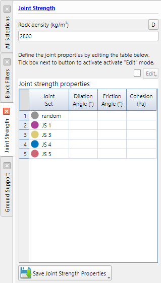
To input the values, tick the Edit checkbox above the joint strength properties table, then enter values into the cells for each joint set.

Dilation angle

Dilation angle may require a brief explanation. DFN joints are perfectly planar, which can result in very long and thin blocks, either flat triangles or thin spikes. These blocks are mathematically removable but are not realistically removable.

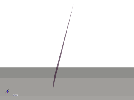
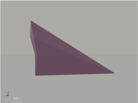
Dilation angle specifies the minimum angle required between the block’s direction of movement and the surface of the joint. That is, as a block slides on the joint plane it must move away from the plane at the dilation angle due to the roughness of the joint.

In the block analyser the direction of movement of blocks is determined by the joint pyramid method of Goodman and Shi (1985). For our tetrahedral blocks, consider the three-sided pyramid formed by the joint surfaces. The direction of movement is the closest line to the direction of gravity that is within the pyramid. This could either be falling, along one joint surface (sliding on one plane), or along the corner line formed by the intersection of two joints (sliding on two planes).

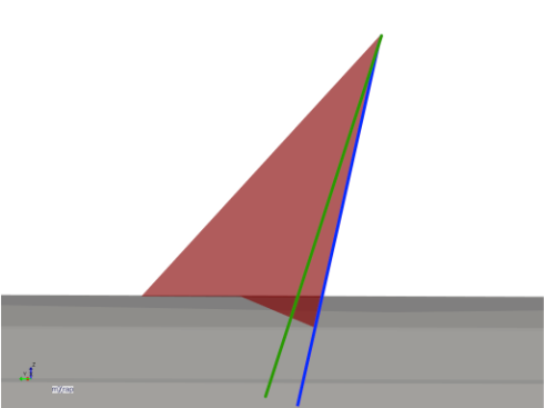
When the block analyser checks removability, it tries to adjust the joint pyramid by the dilation angle of each joint. For example, the joint shown by the blue line in the below image has a dilation angle of 5°, the adjusted plane is shown by the green line. If the joint surfaces are too close together then the adjusted joint pyramid will be empty, and the block is considered not removable and excluded from the analysis.

Friction angle and cohesion

These are the Mohr-Coulomb parameters used in the formulae listed in the Block Stability Calculation section above.

Saving properties

Click the Save Joint Strength Properties to save the current values for the joint strength properties into this project folder. This will allow the values to be restored the next time that you open the project.

This panel provides several filtering options to exclude blocks from the analysis. Typically this is used to remove small or shallow blocks which will come out with the initial blasting, but there are also options to exclude blocks based on their failure mechanism, location, or the joint sets which form them.

${Vb}_{critical}$ is the minimum volume required for a block to be included, in cubic metres. This is used to remove small blocks.
${APH}_{critical}$ is the minimum apex height, defined as the distance from the block’s apex point to the closest point on the excavation surface. This is used to remove shallow blocks.
${Weight}_{critical}$ is the minimum weight required for a block to be included.

The failure mechanism has tickboxes for falling, sliding on one plane, or sliding on two planes. If the option is unticked, then those blocks will be excluded from analysis.

The location options are based on the gradeline height value and the height for backs value. There are tick options that control whether blocks above or below the gradeline are included in analysis, and options that control whether blocks in the backs or walls are included in analysis. The classification is based on the highest point of a block’s free surface on the excavation. For example if the height for backs is 4.0m, and the block’s free surface extends from 3.8m up to 4.1m, then the block’s would be classified as being in the backs.

The joint sets table has ticks for each joint set used in all of the accumulated blocks. If you untick a joint set, then all blocks that contain at least one joint from that joint set will be excluded from the analysis.

The stability options are used only to filter the blocks shown in the 3D view, this allows you to visually inspect only blocks within a certain range of Factor of Safety.

Ground Support Control Panel

In this panel you can tick a ground support standard from your ground support standard designer library. If you are using a simple tunnel geometry then the standard will be virtually installed into the tunnel. Note that the tunnel profile as defined in the support standard should be a close match to the tunnel profile used for the excavation geometry. If there is a mismatch then the system will attempt to move the bolts in or out to pin them to the excavation surface, up to the distance limit specified in the Maximum Distance To Shift Bolts input. When the support is virtually installed, the block stability will be automatically recalculated and all charts and statistics will be updated.

If you do not yet have any ground support standard designs in your library, you can go to the Support Standards window to create a standard.

All Blocks 3D View

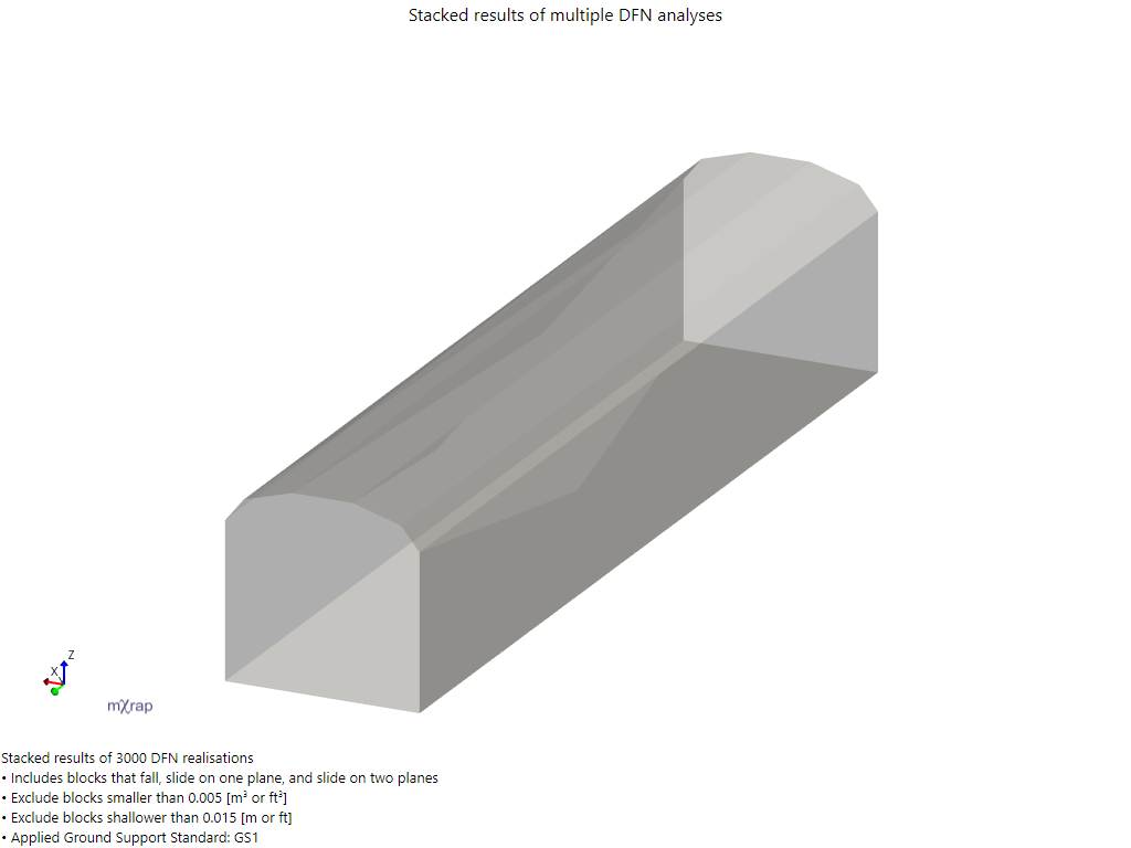
This view allows you to view the excavation surface, the accumulated blocks, and some statistical information about block locations and ground support performance. By default the excavation surface shown is a transparent grey.

Excavation Painted Series

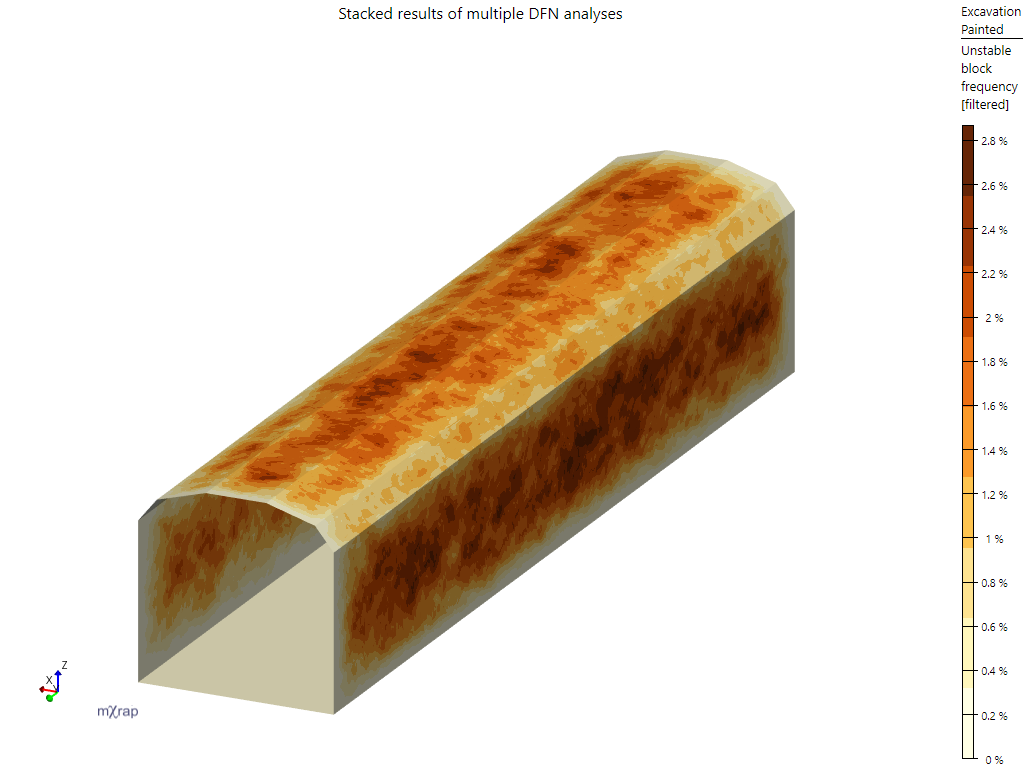
In the series options you can turn off the Excavation Surface series and turn on the Excavation Painted series to get an alternative view of the excavation which shows statistical information about the location of unstable blocks’ free surface areas. Here is the tunnel showing unstable block frequency, defined as the percentage of DFN realisations for which an unstable block’s free surface covered that area of the excavation surface.

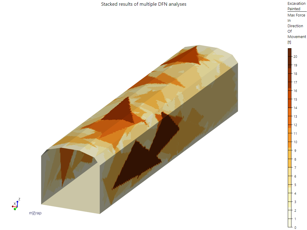
You can also change the colouring option to show the maximum weight of unstable blocks across the excavation surface, or the maximum force in the direction of movement for the blocks (that is the force after taking into account the joint friction for sliding blocks).

Blocks Series

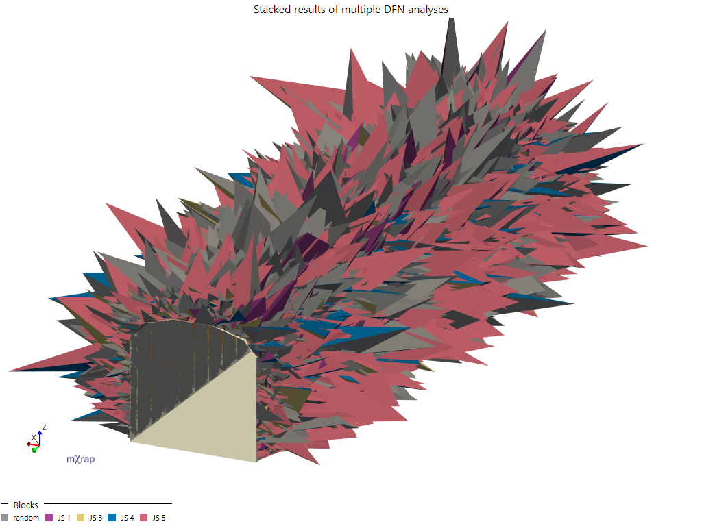
This shows all of the removable blocks passing the current filters. By default the colouring shows the joint sets of the joints that form each block. There are other markerstyle options for block weight, force in direction of movement, and factor of safety.

Bolt Anchorages Series

This series shows thick lines showing the installed bolts for the currently selected ground support standard, coloured according to the total weight per anchored length for the bolt across all DFN realisations. For the block analyser, the anchored length is the length of the bolt that is outside of the block and opposite to the block’s direction of movement, as illustrated in the diagram below.

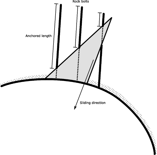
The anchored weight per length is then calculated as the weight of the block divided by the anchored length, and is applied to only the anchored length section of the bolt. Because each bolt will anchor different blocks over the many different DFN realisations, the total anchored weight per length will vary across the bolt. This value is not normalised so you should be careful when interpreting it, as more DFN realisations will naturally result in a higher total value. It is best to use this display as informative of problematic locations and block depths only.

Block Apices Series

This series displays a point on the apex of each block shown in the 3D view. The points can be used with the picking system to investigate a single block for closer analysis, by hovering over the point with your mouse cursor and pressing the F2 button. The picked block will then be displayed in the Picked Block Details display and Picked Block 3D View, discussed later.

Normalising Block Failure Rates

The total number of block failures increases with the number of DFN realisations that are accumulated in a project. The block analyser has two methods of normalising block failure rates so that they can be interpreted more easily, and compared across different project variations (for example, to compare failure rates for different tunnel orientations).

The first method is normalising to a percentage of DFN realisations in which a particular kind of failure occurred. For example, a table might display the percentage of iterations in which at least one block weighing more than 10t failed. This is the most general method of normalisation and allows you to consider the probability of certain events occurring for any kind of excavation geometry. However, if you are analysing a tunnel then the probability of a certain failure occurring is going to increase as the length of your tunnel increases. We will call this the normalised failure rate.

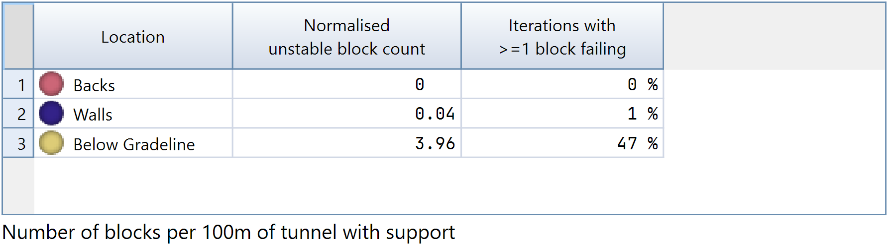
The second method normalises to a number of times that a particular event occurs per 100m of tunnel. This provides a more convenient number to consider the average rate at which something is likely to occur when progressively developing drives. You may see this listed as something like “normalised unstable block count” for the average number of unstable blocks per 100m of tunnel, or “normalised failure count” for the average number of bolt failures per 100m of tunnel. For example, a normalised unstable block count of 0.04 indicates that on average one block fails for every 2.5km of tunnel in these same rock mass conditions and same tunnel orientation, whereas a count of 2 would indicate that on average one block fails every 50m. We will call this the normalised count.

Block Counts By Location Table

This table shows the normalised count and failure rate for blocks, broken down based on the block locations: backs, walls, and below gradeline. This allows you to see the average rate at which unstable blocks occur in each location.

Weight Bin Boundaries Table

This table allows you to specify boundaries used for dividing blocks into weight bins. You can edit the table by ticking the edit checkbox in the top-right. If you want to add a new boundary then click the edit button and choose the insert new row option. As an example, if we define three boundaries: 0.1, 1, and 10, then there will be four weight bins:

<0.1t
0.1t - 1t
1t - 10t
>10t

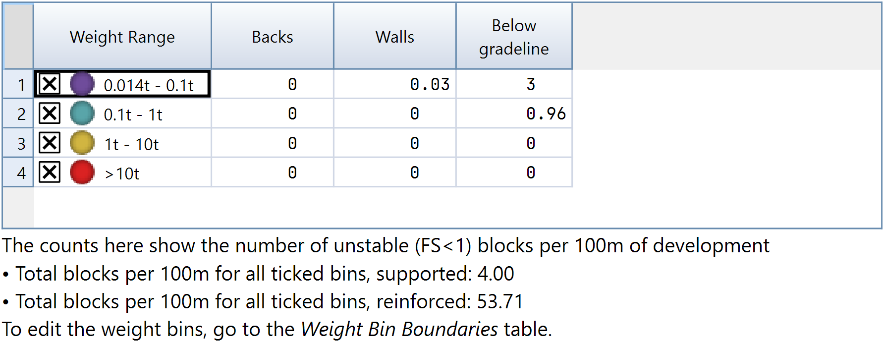
Note that the lowest boundary will typically show a range, in our case it shows 0.014t - 0.1t. The lower part of this range is being automatically filled in based on the minimum volume and weight filter options ${Vb}_{critical}$ and ${Weight}_{critical}$ . In our case ${Vb}_{critical}$ is 0.005, which equates to a minimum weight of 0.014t.

Weight Bin Block Counts By Location Table

This table shows the normalised count for unstable blocks broken down by weight bins and block locations. This allows you to see the average rate at which unstable blocks occur during development for different weight ranges, and roughly where those blocks are occurring.

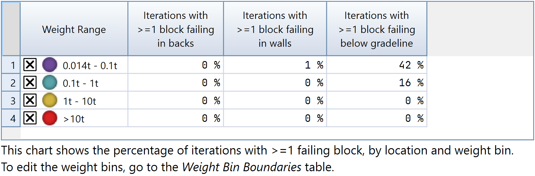
Weight Bin Failure Rate Table

This table shows the normalised failure rate for unstable blocks broken down by weight bins and block locations. This allows you to see the probability of unstable blocks occurring with a fixed kind of excavation surface (e.g. an intersection or a chamber) for different weight ranges, and roughly where those blocks are occurring.

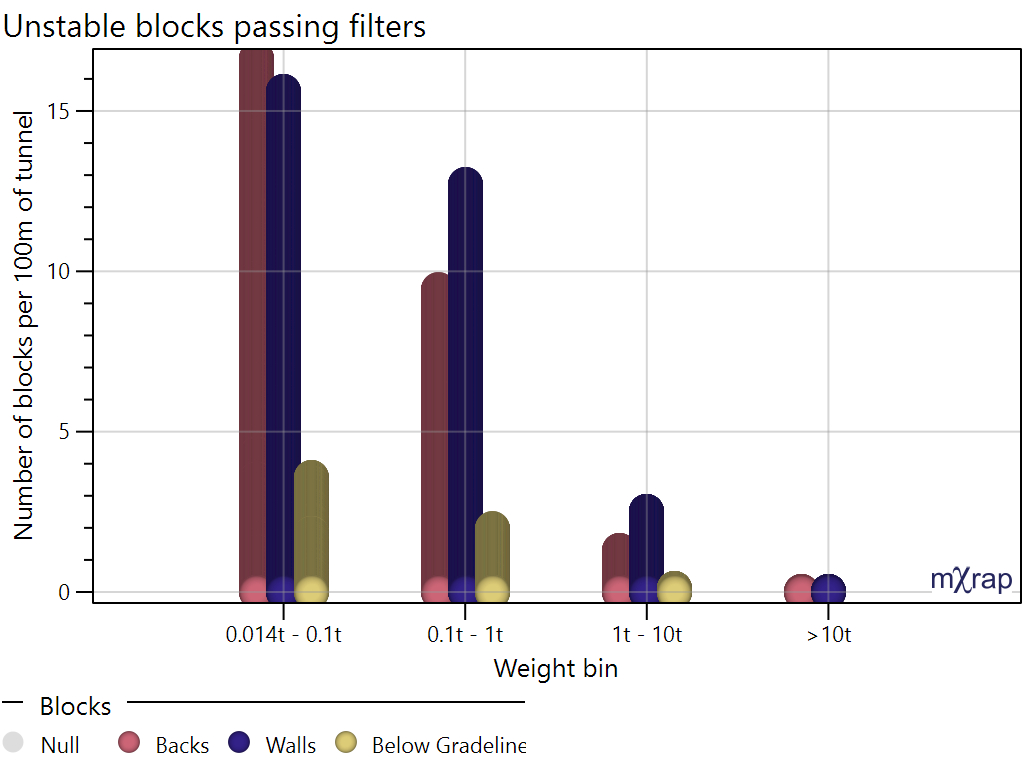
Unstable Blocks Chart

This chart shows a histogram of normalised unstable block counts broken down into weight bins and locations. In the chart’s Controls panel you can adjust the grouping of the chart, by default the primary grouping is the weight bin and the secondary grouping is the block location, as shown below.

Block Weight Distribution Chart

This chart shows a reverse cumulative distribution of block weights. If your excavation is a simple tunnel then the Y axis will be a normalised block count (mean number of blocks per 100m), otherwise it will be the mean number of blocks per DFN realisation.

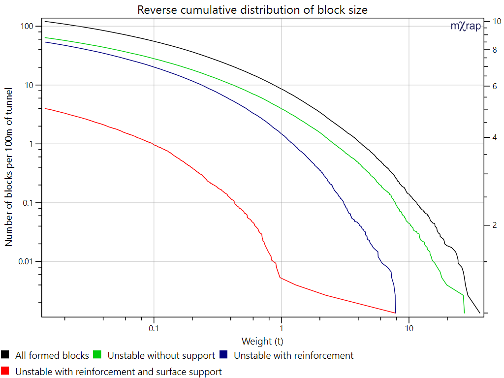
There are four lines. The black line shows all formed blocks passing the current filters (removable blocks). The green line shows the removable blocks which are unstable without support (i.e. unstable considering the joint strength parameters only). The blue line shows the blocks which are unstable with bolts installed. The red line shows the blocks which are unstable with bolts and surface support installed.

Each point on the line shows the number of blocks per 100m of development (the value on the Y axis) which have a weight above or equal to the value on the X axis. For example, if we are considering blocks that weigh >=1t, we find 1 on the X axis. Looking at the green line there are ~4 blocks per 100m that weigh >=1t and are unstable without any support. Looking at the red line, there are only ~0.005 blocks per 100m that weigh >=1t and are still unstable with bolts and surface support.

Block Weight vs FoS Chart

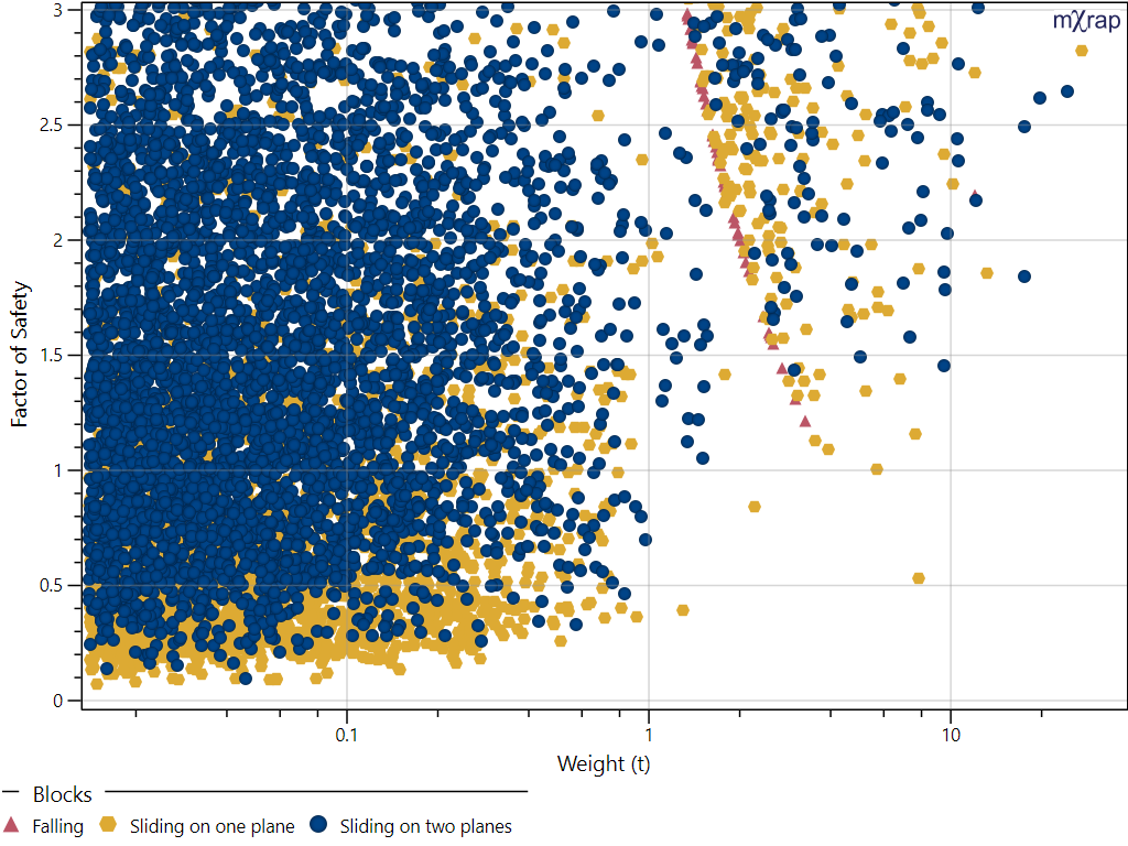
This is a scatter plot showing each block’s weight and factor of safety. The factor of safety axis is capped to a maximum of 3, so any blocks with a higher FoS will not be visible.