Theory

Conceptually, a discrete fracture network (DFN) model is a statistical model that captures the spatial variability of the discontinuity fabric of the rock mass. A DFN model is fully defined by a set of statistical input parameters and the fracture system model (Sewnun et al. 2022). With a single set of input parameters, many different discrete fracture networks can be generated. Each of these DFNs consist of a combination of discontinuities that satisfies the desired statistical parameters. Each DFN, therefore, is a different realisation of the DFN model satisfying the same statistical characteristics defined by that DFN model. The purpose of the DFN model, therefore, is to capture the variability of the discontinuities in a rock mass, leaving the designer to deal only with the uncertainty component (Sewnun et al. 2022).

1. DFN inputs

Block Analyser

📄

Tools for probabilistic assessment of tetrahedral block formation on your excavation geometry, the stability of those formed blocks, and the performance of your ground support standards for supporting those blocks under static conditions.

DFN (Generator)

📄

This app allows you to generate DFN parameters from your structural data and calibrate the DFN parameters with your sampling data.

1.1. Orientation

In geotechnical applications, the orientation of discontinuity data is defined by dip and dip direction. As for the distribution of the discontinuity orientation, it can be quantified by different means. The most popular one, and the one used in the Baecher model, is the Fisher-K value, originally proposed by Fisher (1953) and summarised by Priest (1993), which provides a valuable model due to its simplicity and flexibility (Potvin & Hadjigeorgiou 2020). However, this parameter describes a symmetric distribution; it consequently provides only an approximation for asymmetric data (Priest 1993).

1.2. Size

Discontinuity size is often a critical input into the DFN model and a key parameter for sensitivity studies. Fracture size cannot be directly measured; it is an interpretation of 2D observation data to 3D data. Trace length data act as a footprint for 3D discontinuities as they intersect sampling planes. Trace length may be defined as “the length of a fracture trace formed as the intersection between a fracture and 2D sampling line” (Mauldon & Dershowitz, 2000).

Three main distribution forms have been identified and developed (Dershowitz, 1984):

• Exponential form for trace length distribution
• Lognormal distribution
• Hyperbolically shaped distributional form

Figure: Histogram of joint trace lengths, with best fit exponential and lognormal curves (Priest and Hudson, 1981)

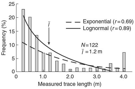
The biases affect the distribution of the trace lengths data and are particularly present in underground mine environments. For instance, a power law size distribution, sampled on the limited exposure of a drift, will in fact be seen as a log-normal distribution (LaPointe et al. 1999). Trace length is subjected to four major biases due to sampling error: orientation bias, size bias, truncation bias, and censoring bias:

• Orientation Bias: The orientation bias occurs when a traverse or a borehole does not perpendicularly intercept the discontinuities (Terzhagi, 1965). Therefore, the measured frequency is lower than the actual perpendicular frequency.
• Size Bias: Longer discontinuities are more likely to be found on the outcrop or rock face and are more likely to be intercepted than smaller joints. Therefore, the measured frequency is lower than the true frequency obtained on a surface of infinite dimensions (Kulatilake et al., 1984). It also influences the average trace length measured on an outcrop (Zhang and Einstein, 1998).
• Truncation Bias: The mapper voluntarily decides to omit discontinuities whose lengths are below a certain predefined threshold. This bias can be neglected if the truncation length is significantly lower than the average trace length (Kulatilake et al., 1984).
• Censoring 21Bias: The surfaces available for mapping are of finite dimensions. It happens that the joints have trace lengths that exceed the available dimensions and that the terminations are not visible, which often happened in mining drives for discontinuity near-vertical. This type of bias tends to underestimate the trace length of discontinuities (Brady and Brown, 2004).

There are some ways to estimate unbiased trace length. For a scanline, the unbiased average trace length (μ) of discontinuities can be estimated using the method cited by Laslett (1982). Window mapping allows to reduce or eliminate some sampling bias in addition to provide higher sampling of an outcrop or wall surface. Some analytical solutions have been developed to estimate unbiased average trace length (μ): Pahl (1981) and Zhang & Einstein (1998).

1.3. Intensity ($P_{32}$)

The term intensity refers to the terminology used by Dershowitz & Einstein (1988): Number of joints per unit area or volume, or total joint trace length per unit area, or total joint area per unit volume. Swenun et al. (2022) explains: “Dershowitz & Herda (1992a) defined a system of fracture intensity measures of different dimensions applicable to a special joint set distribution. This is summarised and modified by Rogers et al. (2017) in Table 1. Fracture intensity measures are referred to as $P_{ij}$, where the subscript i refers to the dimensions of a sample and the subscript j refers to the dimension of measurement. An in-depth discussion of the fracture intensity measures can be found in Dershowitz & Herda (1992a).” The intensity can then be defined by the linear intensity ($P_{10}$), the surface intensity ($P_{21}$) and the volumetric intensity ($P_{32}$).

Table 1. The $P_{ij}$ system of fracture intensity (modified after Roger et al. 2017)

		Dimension	of	measurement
		0 Count	1 Length (m)	2 Area (m2)	3 Volume (m3)
Dimension of sample	1 Length (m)	$P_{30}$ (m-1) No. of fractures per length	$P_{11}$ (m-1) Length of fractures traces per length
	2 Area (m-2)	$P_{20}$ (m-2) No. of fractures per area	$P_{21}$ (m-1) Length of fractures traces per area
	3 Volume (m-3)	$P_{30}$ (m-3) No. of fractures per volume		$P_{32}$ (m-1) Area of fractures per volume	$P_{33}$ (m-1) Volume of fractures per volume

The $P_{10}$ can be estimated from linear surveys such as boreholes (core logging or Televiewer) or scanlines. The $P_{21}$ measurements can be obtained from any area where the discontinuities are systematically mapped (photogrammetry, LiDAR, systematic drift mapping, window mapping, etc.). The $P_{21}$ is the sum of the length of discontinuity traces per area. Although it is not influenced by the sampled area, the orientation of the area generates modifications in the results of $P_{21}$ (Chen, 2010). The $P_{21}$ is then much less affected by orientation bias than $P_{10}$ and can be corrected for.

The preferred method of fracture intensity for the generation of a DFN is $P_{32}$ (fracture area/unit volume) (Rogers et al. 2017). $P_{32}$ is an intrinsic property of the rock mass and cannot be measured in situ (Weir & Fowler 2016). $P_{32}$ can be estimated by multiplying $P_{10}$ and $P_{21}$ with conversion factors (Dershowitz & Herda 1992b; Wang 2005). Since the value of $P_{32}$ cannot be measured directly it needs to be calibrated after initial estimation (Sewnun et al. 2022).

2. Data gathering

To obtain the critical DFN inputs parameters, different survey techniques can be used. Only some techniques offer all the data inputs needed for estimating DFN inputs parameters.

Table 2. Characterization Methods

Characterization Methods	Orientation	Intensity	Size (trace length)
Core logging	✅	✅	❌
Televiewer	✅	✅	❌
Scanline (Line mapping)	✅	✅	✅
Window mapping (Manual)	✅	*Only if systematic measures	✅
Window mapping (LiDAR or photogrammetry)	✅	*Only if systematic measures	*Only if systematic measures
Drift Mapping	✅	❌	*Not full distribution

The quality of a DFN relies heavily on the quality of the field data and its interpretation. Here is some guidance regarding critical data, recommended practises and advanced practice to collect structural data to generate DFN.

Table 3. Critical, recommended and advanced data needed while gathering data for DFN, by data source.

Data Source	Critical data	Recommended practise	Advanced Practice
Along boreholes (Televiewer & core logging)	Boreholes: Location (collar & survey) -Data source Structures: -Dip & dip direction -Distance along the borehole	All Critical data + Boreholes: -Borehole ID -Mapper -Date of mapping Structures: -Structure type -Lithology	All Recommended practise data + Structures: - Aperture -Filling -Roughness
Line mapping (scanline)	Line: -Locality (orientation) -Plunge Structures: -Dip & dip direction -Distance along the traverse	All Critical data + Line: -Line ID -Exact location -Total length -Minimum trace length mapped -Mapper -Date of mapping Structures: -Structure type -Lithology	All Recommended practise data + Line: -Start height from the floor -End height from the floor -Excavation height Structures: -Aperture -Filling -Roughness -Nb of ends visible -Termination type
Area mapping (photogrammetry, LiDAR, manual)	Area: - Locality Structures: -Dip & dip direction -Trace length	All Critical data + Area: -Exact location -Dimension (circle: radius; rectangle: height and width; tunnel: idealized tunnel shape or scan of excavation) - Area ID -Minimum trace length mapped - Mapper -Date of mapping Structures: -Location XYZ (start or middle) -Structure type -Lithology	All Recommended practise data + Structures: -Aperture -Filling -Roughness -Nb of ends visible -Termination type
Others		Geotechnical Domains